Unconstrained optimization: L-BFGS and CG

About algorithms

ALGLIB package contains three algorithms for unconstrained optimization: L-BFGS, CG and Levenberg-Marquardt algorithm. This article considers first two algorithms, which share common traits:

1. they solve general form optimization problem (target function has no special structure)
2. they need function value and its gradient only (Hessian is not needed)
3. both algorithms support numerical differentiation when no analytic gradient is supplied by user

L-BFGS algorithm

L-BFGS algorithm builds and refines quadratic model of a function being optimized. Algorithm stores last M value/gradient pairs and uses them to build positive definite Hessian approximation. This approximate Hessian matrix is used to make quasi-Newton step. If quasi-Newton step does not lead to sufficient decrease of the value/gradient, we make line search along direction of this step.

Essential feature of the algorithm is positive definiteness of the approximate Hessian. Independently of function curvature (positive or negative) we will always get SPD matrix and quasi-Newton direction will always be descent direction.

Another essential property is that only last M function/gradient pairs are used, where M is moderate number smaller than problem size N, often as small as 3-10. It gives us very cheap iterations, which cost just O(N·M) operations.

Nonlinear conjugate gradient method

Unlike L-BFGS algorithm, nonlinear CG does not build quadratic model of a function being optimized. It optimizes function along line, but direction to explore is chosen as linear combination of current gradient vector and previous search direction:

x_k+1 = x_k + α_kd_k
d_k+1 = -g_k+1+β_kd_k

α is chosen by minimization of f(x_k+α_kd_k). There are exist several formulae to calculate β, each of them corresponding to distinct algorithm from CG family. Such approach, despite its simplicity, allows to accumulate information about function curvature - this information is stored in the current search direction.

Comparison of L-BFGS and CG

From the user's point of view these algorithms are very similar: they solve unconstrained problems, need function gradient, have similar convergence speed. It makes them interchangeable - if your program uses one algorithm, it can switch to another one with minimal changes in the source code. Both methods can be used for problems with dimensionality ranging from 1 to thousands and even tens of thousands.

However, differences exist too:

• computational overhead of the L-BFGS iteration is larger than that of CG. Hence nonlinear conjugate gradient method is better than L-BFGS at optimization of computationally cheap functions.
• from the other side, one iteration of L-BFGS usually needs less function evaluations than CG (sometimes up to 1.5-2 times less). Hence L-BFGS is better at optimization of computationally expensive functions.
• On extremely ill-conditioned problems L-BFGS algorithm degenerates to the steepest descent method. Hence good preconditioner is needed to remedy this. Nonlinear CG retains its key properties independently of problem condition number (although convergence speed decreases on ill-conditioned problems).
• methods behave differently when preconditioner is changed during optimization process. Nonlinear conjugate gradient method loses all information about function curvature accumulated so far. Recommended strategy - infrequent updates on significant curvature changes. Too frequent updates will make method degenerate into steepest descent algorithm with all its drawbacks. Contrary to its counterpart, L-BFGS algorithm allows to change preconditioner without loosing information about function curvature. Recommended strategy - update as frequent as needed.
• convergence theory for nonlinear CG is better studied than that of L-BFGS. Nonlinear CG converges when gradient is Lipschitz continuous (not necessarily twice continuously differentiable). As for L-BFGS, only convergence on twice continuously differentiable functions, strictly convex at extremum, was proved.

Performance

We've used following settings to compare different optimization algorithms:

• test function - generalized Rosenbrock
• problem size - in 10...100, with step 10.
• initial point - x = [-1, -1, ..., -1].
• stopping conditions - gradient norm is less than 10^-8.
• CPU used -Intel Core 2 Q6600, running at 2.4 GHz
• OS used - 32-bit Ubuntu
• compiler - GCC, with maximum optimization settings
• each algorithm made 10 runs

Comparison of algorithms from ALGLIB

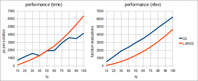
In the first part of our experiment we've compared performance of ALGLIB implementations of CG and L-BFGS (with m=8). We've got following results:

Following conclusions can be made. First, when measured in function evaluations, CG is inferior to L-BFGS. However, this drawback is important only when function/gradient are hard to compute. But if function and its gradient are easy to compute, CG will be better than L-BFGS.

Comparison with other packages

In the second part of experiment we've compared ALGLIB implementation of CG with CG from GNU Scientific Library (GSL). We've used GSL 1.12 (version shipped with OS). GSL includes two kinds of CG: PR (Polak-Ribiere) and FR (Fletcher-Reeves). We've tested our implementation against CG-PR because it has somewhat better performance. On the charts below you can compare performance of ALGLIB and GSL.

ALGLIB was 7-8 times faster than GSL - both in computational time and in function evaluations. But why difference is so high? First, ALGLIB uses more efficient line search algorithm. Second, ALGLIB includes modern version of CG algorithm while GSL uses obsolete and inefficient FR and PR variants.

Just to be sure that such huge difference is not an error, we've made additional tests. Another CG algorithm from GSL (FR-CG) was even worse - ALGLIB CG was 15-20 times faster than FR-CG. We've tried to use another test function, but got similar results. Finally we've tried more stringent stopping conditions - |g|<10^-14 instead of |g|<10^-8. To our surprise, GSL CG failed to converge while ALGLIB CG have correctly converged.

Starting to use algorithm

Choosing between analytic and exact gradient

Before starting to use L-BFGS/CG optimizer you have to choose between numerical diffirentiation or calculation of analytical gradient.

Both algorithm - L-BFGS and CG - need function gradient. For example, if you want to minimize f(x,y)=x²+exp(x+y)+y², then optimizer will need both function value at some intermediate point and function derivatives df/dx and df/dy. How can we calculate these derivatives? ALGLIB users have several options:

1. gradient is calculated by user, usually through symbolic differentiation (so called analytical or exact gradient). This option is the best one because of two reasons. First, precision of such gradient is close to the machine ε (that's why it is called exact gradient). Second, computational complexity of N-component gradient is often only several times (not N times!) higher than calculation of function itself (knowledge of the function's structure allows us to calculate gradient in parallel with function calculation).
2. gradient is calculated by ALGLIB through numerical differentiation, using 4-point difference formula. In this case user calculates function value only, leaving all differentiation-related questions to ALGLIB package. This option is more convenient than previous one because user don't have to write code which calculates derivative. It allows fast and easy prototyping. However, we can note two significant drawbacks. First, numerical gradient is inherently inexact (even with 4-point differentiation formula), which can slow down algorithm convergence. Second, numerical differentiation needs 4·N function evaluations in order to get just one gradient value. Thus numerical differentiation will be efficient for small-dimensional (tens of variables) problems only. On medium or large-scale problems algorithm will work, but very, very slow.
3. gradient is calculated by user through automatic differentiation. As result, optimizer will get cheap and exact analytical gradient, and user will be freed from necessity to manually differentiate function. ALGLIB package does not support automatic differentiation (AD), but we can recommend several AD packages which can be used to calculate gradient and pass it to ALGLIB optimizers:
   • AutoDiff for C#
   • FuncDesigner for Python
   • FADBAD++ for C++

Depending on the specific option chosen by you, you will use different functions to create optimizer and start optimization. If you want to optimize with user-supplied gradient (either manually calculated or obtained through automatic differentiation), then you should:

• create optimizer with minlbfgscreate (mincgcreate) function
• pass callback calculating function value and gradient (simultaneously) to minlbfgsoptimize (mincgoptimize). If you erroneously pass callback calculating function value only then optimizer will generate exception on the first attempt to use gradient.

If you want to use ALGLIB-supplied numerical differentiation, then you should:

• create optimizer with minlbfgscreatef (mincgcreatef) function. This function accepts one additional parameter - differentiation step. Numerical differentiation is done with fixed step. However, step size can be different for different variables (depending on their scale set by minlbfgssetscale/mincgsetscale call).
• pass callback calculating function value (but not gradient) to minlbfgsoptimize (mincgoptimize). If you erroneously pass callback calculating gradient then optimizer will generate exception.

Tuning algorithm parameters

L-BFGS algorithm is quite easy to tune. The only parameter to tune is number of correction pairs M - number of function/gradient pairs used to build quadratic model. This parameter is passed to the function which is used to create optimizer object. Increase of M decreases number of function evaluations and iterations needed to converge, but increases computational overhead associated with iteration. On well-conditioned problems M can be as small as 3-10. If function changes rapidly in some directions and slowly in other ones, then you can try increasing M in order to increase convergence.

As for nonlinear conjugate gradient method, it has no tunable parameters. You just call mincgcreate function, which creates optimizer, and that's all.

Scale of the variables

Before you start to use optimizer, we recommend you to set scale of the variables with minlbfgssetscale or mincgsetscale functions. Scaling is essential for correct work of the stopping criteria (and sometimes for convergence of optimizer). You can do without scaling if your problem is well scaled. However, if some variables are up to 100 times different in magnitude, we recommend you to tell solver about their scale. And we strongly recommend to set scaling in case of larger difference in magnitudes.

We recommend you to read separate article on variable scaling, which is worth reading unless you solve some simple toy problem.

Preconditioner

Preconditioning is a transformation which transforms optimization problem into a form more suitable to solution. Usually this transformation takes form of the linear change of the variables - multiplication by the preconditioner matrix. The most simple form of the preconditioning is a scaling of the variables (diagonal preconditioner) with carefully chosen coefficients. We recommend you to read article about preconditioning, below you can find the most important information from it.

You will need preconditioner if:

• your variables have wildly different magnitudes (thousand times and higher)
• your function rapidly changes in some directions and slowly - in other ones
• analysis of Hessian matrix suggests that your problem is ill-conditioned
• you want to accelerate optimization

Sometimes preconditioner just accelerates convergence, but in some difficult cases it is impossible to solve problem without good preconditioning.

ALGLIB package supports several preconditioners:

• default one, which does nothing (just identity transform). It can be activated by calling minlbfgssetprecdefault or mincgsetprecdefault.
• diagonal Hessian-based preconditioner. In order to use this preconditioner you have to calculate diagonal of the approximate Hessian (not necessarily exact Hessian) and call minlbfgssetprecdiag (or mincgsetprecdiag) function. Diagonal matrix must be positive definite - algorithm will throw an exception on matrix with zero or negative elements on the diagonal. This preconditioner can be used for convex functions, or in situations when function is possibly non-convex, but you can guarantee that approximate Hessian will be positive definite.
• diagonal scale-based preconditioner. This preconditioner can be turned on by minlbfgssetprecscale (or mincgsetprecscale) function. It can be used when your variables have wildly different magnitudes, which makes it hard for optimizer to converge. In order to use this preconditioner you should set scale of the variables (see previous section).

Stopping conditions

ALGLIB package offers four kinds of stopping conditions:

• gradient-based - scaled gradient norm is small enough (scaled gradient is a gradient which is componentwise multiplied by vector of the variable scales)
• stepsize-based - scaled step norm is small enough (scaled step is a step which is componentwise divided by vector of the variable scales)
• function-based - function change is small enough
• iteration-based - after specified number of iterations

You can set one or several conditions by calling minlbfgssetcond (mincgsetcond) function. After algorithm termination you can examine completion code to determine what condition was satisfied at the last point.

We recommend you to use first criterion - small value of gradient norm. This criterion guarantees that algorithm will stop only near the minimum, independently if how fast/slow we converge to it. Second and third criteria are less reliable because sometimes algorithm makes small steps even when far away from minimum.

Note #1
You should not expect that algorithm will be terminated by and only by stopping criterion you've specified. For example, algorithm may take step which will lead it exactly to the function minimum - and it will be terminated by first criterion (gradient norm is zero), even when you told it to "make 100 iterations no matter what".

Note #2
Some stopping criteria use variable scales, which should be set by separate function call (see previous section).

Running algorithm

After creation and tuning of the optimizer object you can begin optimization using minlbfgsoptimize (mincgoptimize) function. It accepts as parameters optimizer object and callbacks which calculate function/gradient. Optimization result can be obtained using minlbfgsresults (mincgresults) function.

Examples

In order to help you use L-BFGS and CG algorithms we've prepared several examples. Because these algorithms have similar interface, for each use case we've prepared two identical examples - one for L-BFGS, another one for CG.

• minlbfgs_d_1 (mincg_d_1) - this example shows how to minimize function with L-BFGS or CG.
• minlbfgs_d_2 (mincg_d_2) - this example shows how to use upper limit on step size and efficient restarts.
• minlbfgs_ftrim (mincg_ftrim) - this example shows how to minimize function with singularities at the domain boundaries. This example is discussed in more details in another article.
• minlbfgs_numdiff (mincg_numdiff) - this example shows how to minimize function using numerical differentiation.

We also recommend you to read 'Optimization tips and tricks' article, which discusses typical problems arising during optimization.

This article is licensed for personal use only.